LET'S REPAIR AND MODERNIZE THE SHARPE RATIO

Since first published by Harry Markowitz in 1952, millions of investors, directly or through their advisors or portfolio managers, have relied upon a particular analysis of portfolio risk and returns to make their investment decisions.  Modern Portfolio Theory (MPT), and its components (mean return, variance, beta, etc.) are widely-accepted as the state of the science in portfolio management, but there are critical flaws in the method that must be addressed.  CrystalBull’s live timing stack is built around the same problem — scoring return versus variability in a way you can actually trade. See the market timing dashboard and long-run model returns.  Herein, we attempt to solve a few of the fundamental issues with MPT and its most popular measure, the Sharpe Ratio:

1.  Average (arithmetic mean) of returns can be highly misleading.
   
2.  Variance and standard deviation are not identities of, nor analogies for, risk.
   
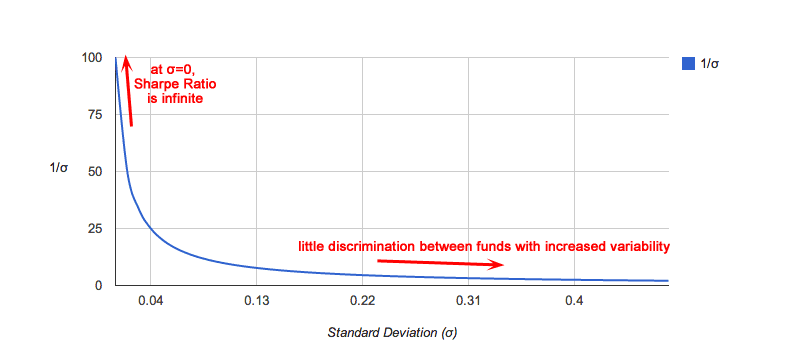
3.  Placing two measurements into a ratio can be distortive.  Changes in the numerator (mean returns) move the ratio linearly, while changes in the denominator (standard deviation of returns) move the ratio hyperbolically.  This leads to a sometimes unhelpful bias to funds with lower returns and lower variance.  A fund with no variability of returns, has an infinite Sharpe Ratio, regardless of return.  That is not helpful to the analysis.
   
4.  A comparison to an index may yield misleading results, as any negative correlation, which may be desirable for the investor, increases the variance, thus lowering the Sharpe Ratio.  A comparison to a risk-free investment does not have this limitation, as such typically has no variance.
   

Let's dive in.

First introduced by William F. Sharpe in 1966, the Sharpe Ratio is a measure of the expected return (reward) of an investment, versus the amount of variability (MPT proxy for risk) in the return.  Since its revision in 1994, the Sharpe ratio has taken on 2 general forms: the ex-ante (prediction of future return and variance), and ex-post (analysis of past return and variance).  For the most part, ex-ante predictions are simply hopeful guesses, or estimates patterned after observations of past performance of similar investment vehicles.  In either case, ex-post observations are the most critical determinations in constructing the Sharpe Ratio.  For that reason, we will focus here on the ex-post Sharpe Ratio.

Let's walk through the derivation of the Sharpe Ratio.  (Don't be discouraged if you don't understand the mathematics;  We'll try to explain as we go along.)  The ex-post Sharpe Ratio measures how high the returns were, versus how varied those returns were.  More specifically, it is the ratio of the differential returns (difference between the returns of the investment and a benchmark investment) versus the historic variability (as standard deviation) of those returns.  Some select a "risk-free" investment (treasury bond) as the benchmark, while others choose an index like the S&P 500.  Because an index of securities has its own variability, which, in calculating the difference of returns, are indistinguishable from the variability of the fund, we choose to use the risk free rate in our study.  Here is the Sharpe Ratio derivation [from Sharpe, 1994], then explanation below:



Why did we go through this exercise?  We wanted to show you the components of the Sharpe Ratio, and how it is constructed, so we can then demonstrate our methods for improving it.  To calculate the Sharpe Ratio, one must first calculate the returns per sub-period of the investment, compare them to a benchmark during the same sub-period, and calculate the difference.  Then, the average of the differences is divided by the standard deviation (variability, or noise) of those differences.  For example, let's say one wanted to calculate the Sharpe Ratio for a fund over one year, and uses the monthly returns for the sub-periods.  In a spreadsheet, one would put the monthly returns of the fund in one column, the monthly returns of the benchmark investment in another column, and calculate the difference between the two for a third column.  Using this column of differences, one would find the average and the standard deviation, and calculate the ratio.  It is far more simple than it appears in the mathematics above;  Most spreadsheet programs will calculate the mean and standard deviation for you.

Why is this a potential problem?  First, because a simple arithmetic mean (average) of return percentages can be misleading.  Return percentages are not additive.  For example, consider the following funds:


These two funds would be indistinguishable were one only to look at the average returns.  However, the realized returns are quite different.  At the end of these four periods, the total return of Fund #1 is -1.25% ((1.10 * 1.05 * 0.95 * 0.90) - 1), while the total return for Fund #2 is -85.75% ((1.90 * 1.50 * 0.50 * 0.10) - 1).  In neither case does the average return reflect a losing investment, nor make any distinction between these two quite different funds.  Simple arithmetic averages, when dealing with return percentages, can be wildly inaccurate.

Consider these funds:
All 3 funds have identical Sharpe Ratios!  Funds A and B have identical average differential returns, as well as identical standard deviations.  Fund C has 1/10th the average returns, and 1/10th the standard deviation of returns.  Because the Sharpe arithmetic has used simple arithmetic means, we are unable to distinguish between these vastly different fund performances.  Click here to view the spreadsheet used for these calculations.

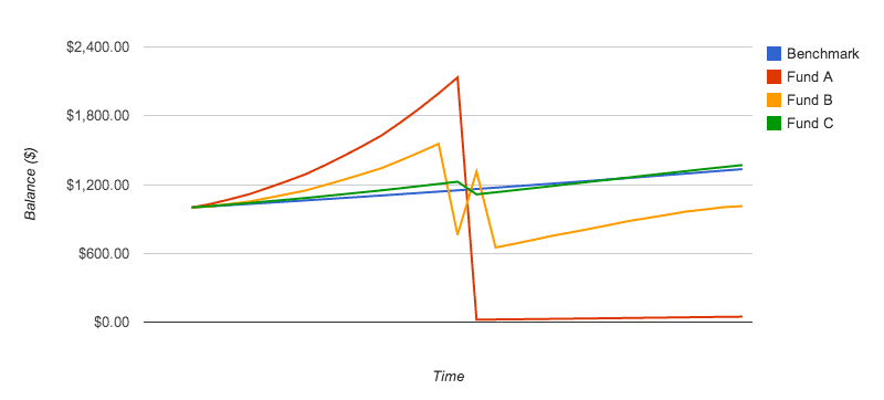
Our solution to this problem is outlined below, but let's continue identifying issues that need to be addressed...

Consider these funds:
Which fund would you prefer?  At no time did Fund A outperform Fund B, yet Fund A has a Sharpe Ratio 3 times higher than that of Fund B.  Click here to view spreadsheet.  A fund manager using the Sharpe Ratio as the sole selection criterion would pass on Fund B.  While there may be value in limiting variability in one's account, this example highlights the problem with using a ratio as a metric.  Changes in the numerator (return) move the ratio linearly, while changes in the denominator (standard deviation) move the ratio hyperbolically.  This places a much higher emphasis on low variability than on higher returns.  That may not be in the investor's best interest.  In practice, we track that tradeoff with dedicated volatility and trend tools, including the CrystalBull Vixen (VIX), Matador, and Trend indicators.

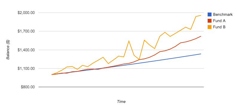
As an aside, an investor could choose two high-return, high-variability funds that are negatively correlated.  That would have the benefit of adding return to the portfolio, while counterbalancing variability.  Reliance on the Sharpe Ratio alone does not facilitate selection of such funds.

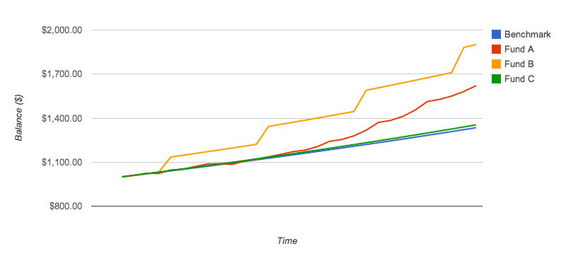
Consider these funds:
Which fund would you rather own?  Which shows more risk?  Fund A has very low variance, so a very high Sharpe Ratio, 33x that of Funds B and C.  Funds B and C have identical Sharpe Ratios.  Why would Funds B and C have Sharpe Ratios less than Fund A?  Fund B has accelerating returns, which appear as variability in the analysis.  Fund C initially has higher returns, but the returns decelerate over time, which also appears as variability in the distribution of returns.  Click here to view spreadsheet.  Here, again, the Sharpe Ratio arithmetic misleads the investor into choosing Fund A over the superior performing, and perhaps less risky, Fund B.

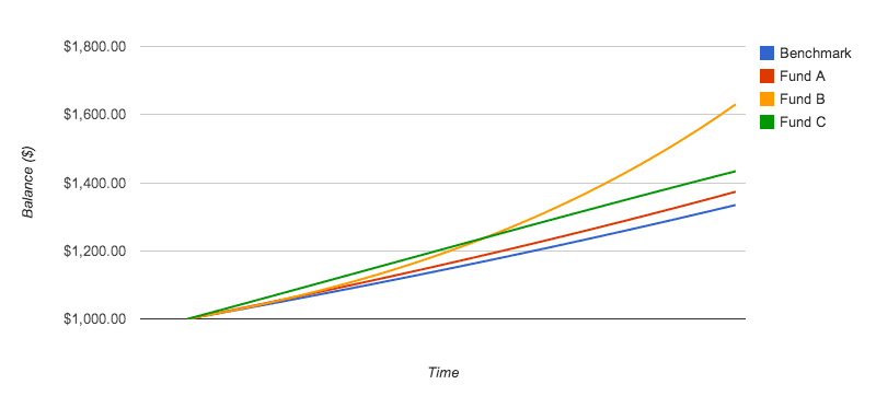
This serves as a nice segue into another issue, so let's get this out of the way:

Variability is not an identity for, nor an analogy to, risk.  Consider these funds:
All 3 funds have an identical distribution of returns.  Fund A's periodic returns are random.  Fund B has the identical periodic returns, but they have been arranged in accelerating order.  Fund C, in decelerating order.  Of course, they all have the identical Sharpe Ratio, as variance and standard deviation have no regard for order.  Click here to see spreadsheet for these funds.

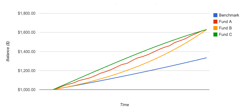
Which of these funds would be most favorable going forward?  Which is most risky?  Many investors believe that, during short sample periods, returns are random, with prices moving in Brownian motion fashion.  Thus, each of the returns shown would be equally likely, alternative histories, with the same probability of occurrence.  As such, they would be indistinguishable from one another, as far as probability of returns going forward, and each would have the same risk.  But, is that truly the case?

Over time, prices and returns are not random;  They are intentional.  Countless man-hours are invested daily in efforts to increase capital, asset, and security prices.  Without correlating results, humankind would have stopped producing long ago.  Fund A's returns appear healthy, and its variability could be explained by seasonality, temporary changes in the marketplace, or randomness.  Fund C's returns could also be random.  However, knowing that the executives and employees of the companies in that fund are making every effort to grow earnings, the declining rate of returns is troubling.  Despite their best intentions, it appears that they are failing to grow returns consistently.  It is not unsound reasoning to reject Fund C, especially since funds with more favorable growth trends are available.  Fund B appears to be most healthy. The efforts of its participants are succeeding in moving rates of return higher.  Thus, in light of the possibility of a random walk, Brownian motion of returns, Fund B has the favorable characteristic of successful growth, and should be selected.

In any case, the increasing rate of return manifests itself as variance in the Sharpe Ratio, and variance is a proxy for risk in the Markowitz mean-variance paradigm.  This flavor of variability should be considered less risky, not more so.  Accounting for second-order, rates of change of returns, is beyond the scope of this paper, reserved for a future follow-up.  The purpose of showing this comparison is to highlight how funds of different characteristics can have identical average and standard deviation of returns.

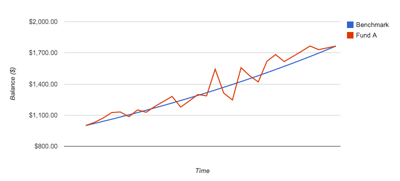
Let's consider another set:
Which fund would you rather own?  The Sharpe Ratios of these funds increase as their returns diminish.  Fund C has an infinite Sharpe Ratio, as its variability is zero.  Fund A's Sharpe Ratio is 50% higher than that of Fund B.  Again, this is because of the hyperbolic weighting of the variability.  Is Fund B more risky than Fund A?  While Fund B has a higher statistical variability than Fund A, all of the changes in variability have been to the upside!  That is not a characteristic of risk.  Click here to see the spreadsheet used for this chart.  A cousin to the Sharpe Ratio, the Sortino Ratio, attempts to correct this by limiting the variability to only those variations to the downside, or below a threshold.  This is an improvement, but does not solve the fundamental issue that variability is not the same as risk.  Here is an example of what analysts might consider a stable, low-variability, low-risk stock:

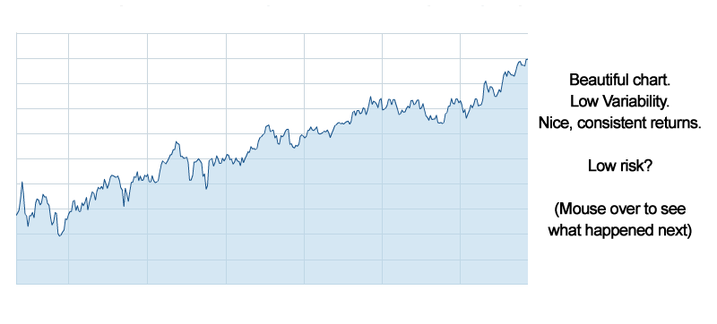
 We could show many more examples of where the standard deviation of sub-periodic returns is a poor proxy for risk, but let's continue...

Any solution we find should accomplish the following:

1) Use a more accurate description of historic returns than the simple arithmetic mean (the numerator).
2) Find a more helpful characterization of risk than the standard deviation of past periodic returns (the denominator).

A simple solution to address the issue with average returns above is to use compound returns.  Instead of adding each periodic return from t=1 to T, we could just take the compound return at the end of the total period (t=T).  Problem solved?  Each fund or security would be scored linearly with its total compound return over the period.  However, we would like to provide a scoring method which lends itself for ex-ante decisions, where we may want to match periodic returns to variance, or to use a Monte Carlo mechanism to determine probabilistic returns.  For this reason, we want to keep the granularity of sub-periodic returns.

Calculating simple returns as we have done above is easy:

However, as we have seen above, periodic returns are not additive;  Adding returns for multiple periods does not yield the total return over the total length of time.  To find the total return over the period $T$, we need to compound the growth for each sub-period, as shown here:

If each return $R_x$ were identical, we could write this is a simplified exponential form: Most of us have seen this arithmetic before.  Over time, returns compound in an exponential fashion.  But, the Return in each sub-period is rarely identical, so compounding in this manner is impossible.  A better method would allow us to use sub-periodic returns to determine the compounded return of exponential growth.  For this reason, we turn our attention to logarithmic returns.

Logarithmic returns measure the rate of exponential growth.  Instead of measuring the percent of price change for each sub-period, we measure the exponent of its natural growth during that time.  Later, we can add each sub-period's exponential growth to get the total growth for the period.    The arithmetic for a single period then becomes:

Again, don't get lost in the arithmetic here...  All we have done is to model price movements based on exponential growth, instead of the simple arithmetic fractional ($P_f/P_i$) percentage growth each period.  Such a fraction has no accounting for how the price went from $P_i$ to $P_f$, other than to say it moved fractionally, in one quantum jump.  Using our log return method, we model the price as having been compounded continually at the rate of $ln(P_f/P_i)$, in an exponential curve.  Recording the growth rates logarithmically, defining the growth curve for the entire time $T$, has some conveniences, such as the ability to add sub-periodic returns, as we shall see below.

To sum logarithmic returns over several periods:

or,

Using rules for logarithms, this expands to:

The astute observer will notice that after all of the intermediate $ln()$s cancel out, we are left with just:

or, We have just proven that logarithmic returns are additive, that the logarithmic return for a period $T$ is equal to the sum of the logarithmic returns for each sub-period $t$.  And, because the logarithmic returns are additive, the arithmetic mean of log returns is much more informative: the average log return, times the number of sub-periods, tells us the exact total compounded return over the period of study.  This solves the problem demonstrated in the Sharpe Ratio analysis above, where average arithmetic returns can be misleading.  Our numerator can now score funds precisely according to total compounded returns.

So, an improved numerator would be the average (arithmetic mean) of logarithmic returns:



This gives us a good weighting of the total compounded return for the period.

In practice, it would be helpful if this measure appeared in our metric as the more commonly relatable annual return percentage.  Investors simply are not familiar with judging sub-periodic returns, especially in logarithmic terms.  For this reason, we normalize our return metric to an average annual return, as follows:



Substituting logarithmic returns for simple arithmetic returns is an effective, easy-to-implement solution to the problems described in the numerator.  This normalized return should be far more helpful to an investor than an average, sub-periodic, arithmetic return.  Our improved numerator is this normalized total return, computed by adding the sub-periodic logarithmic returns, and converting to an annualized return.

What are we missing?  Notice the lack of reference to any benchmark fund.  This approach may obviate the need for a separate benchmark fund in the analysis.  In most cases, a risk-free fund serves simply as a zero, or near-zero, variability baseline from which to measure the variability of the fund under study.  The mean logarithmic return demonstrates the zero-variability baseline for a fund of the same total return over the period.  We can now measure variability of a fund's returns against its own average log return, as we will demonstrate below.  Of course, one could still compare the sub-periodic log returns to the log returns of an external benchmark, if desired.

Consider this fund:



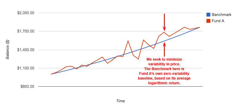
In this case, the benchmark for zero-variability is simply the same fund, had it remained at its average logarithmic rate of return for each period.  This is an important characteristic as we move to solve the issues with the Ratio's denominator.

In a market where prices are set by crowds, variability is inevitable.  Price variability may not be a good indicator of risk, but, should an investor seek to reduce variability?  Overall return is the objective, and minimization of risk is, of course, also an objective.  The risk/reward ratio is an important consideration in every investment decision.  But most risk is, after all, unknowable.  Do we simply find the most convenient proxy we can find for risk (variability), and use it in our decision-making?  Variability looks scary, so should we try to avoid it?  The answer may be "Yes".

But, notice we are discussing variability in Price, not variability in Returns.  This is an important distinction.  The standard deviation of returns does not always properly measure the variability of price, which is our goal.

Why measure variability of price and not returns?  Consider these funds:

Funds A and B have identical periodic returns, identical standard deviation of returns, and, thus, the same Sharpe Ratio.  But, the order of the periodic returns has been rearranged, so that Fund B's price deviates much further from their zero-variance baseline.  Fund A appears much more consistent, and consistency of returns is what most investors seek. In our observations, wild price swings cause many investors to panic, and sell at the drops, or throw caution to the wind, purchasing at the highs of the price spikes.  Both decisions are based on fear; The panic sale is based on the fear of losing, while the jump-on-the-bandwagon purchase is based on the fear of "missing out".  Both of these emotional decisions are unhealthy, and cause some investors to buy high and sell low.  In the example above, Fund B spends some time below the Benchmark fund, and is heading lower.  There is a good chance that many investors would sell the fund here (sell low), missing future returns.  So, to the extent that price variability may lead an investor's decision-making prowess astray, we seek to minimize it.  Thus, we abandon the standard deviation of returns here, and focus on variability in prices.

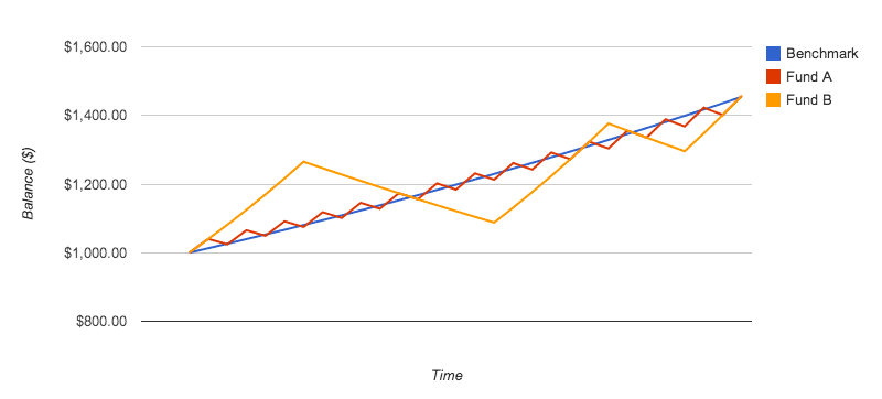
So, is the answer to simply substitute the standard deviation of price for the standard deviation of returns?  Not so fast.

First, it is not the standard deviation of nominal prices that we seek to measure.  A high growth fund will, by definition, have a high variability of price, while the only fund with zero variance will be a fund with zero return.  What we must measure is the variability of the fund's price compared to the ideal: a fund with zero variability.  Fortunately, by measuring the fund's logarithmic returns, we already have a zero-variability baseline for comparison: the same fund's periodic prices, had it earned it average logarithmic return during each sub-period, as discussed above.  An elegant solution obviates the need for a separate benchmark fund, and uses its own zero-variability ideal as the benchmark, as shown here:

The zero-variability price at the end of any period becomes:


The differential we want to measure is $P_n - P_n'$.  But, so that we can compare funds at varying asset prices, we normalize this price differential to a ratio of the zero-variability price: $(P_n - P_n')/P_n'$, as follows



So, we can calculate the standard deviation of this differential ($σ_D$)  over the entire period, as follows:



This standard deviation of price differentials provides more information than the standard deviation of arithmetic returns, especially if one uses variability as a proxy for risk.  How far the price deviates from the ideal is far more important than a single sub-period's return.

Another advantage of this method is consistency across sub-periods of different length.  When measuring the standard deviation of returns, the numbers are much smaller in shorter time periods than in longer.  For example, the standard deviation of a fund using monthly returns will be many times higher than the standard deviation of daily returns.  By measuring the standard deviation of price differentials, the difference in nominal prices for a day is similar in scale to the monthly or yearly price.   Thus, the standard deviation numbers are more relatable, and less dependent on the time granularity chosen.

We now have a more valuable gauge of variability vis-a-vis risk.  But, we still have one problem:

Changes in the denominator move any ratio hyperbolically, obfuscating important information.  As variability (as $σ$) goes to zero, the ratio becomes infinite, regardless of its return.  Once variability increases past a certain point, the ratio provides less information about comparative variabilities between funds.

The following chart demonstrates how changes in the Standard Deviation of returns, in the denominator, affects the Sharpe Ratio.

Furthermore, the rate at which the ratio value falls with rising $σ_R$ is not ideal.  Our observations in behavioral economics have told us that investors as a herd will not react much to small to moderate variability;  In fact, they expect it.  But, with high levels of volatility, they may react, rationally or emotionally, to change investment positions.  This can doom a portfolio to the buy high, sell low failures discussed earlier.  Our Ratio should evaluate accordingly.  Ideally, the variability factor will attenuate our measure slightly as variability grows from zero, then at a greater and greater pace as variability increases.  Our preferred weighting is nearly the opposite of the Sharpe weighting.

If we structure the variability component of our measure to range from $0 → 1$, we could use this component as weighting multiplier (instead of divisor), and our measure would retain important information about the Return Rate, mapping closely to expected future returns.  One way to accomplish a variability factor range between $0$ and $1$ would be to compare the standard deviation of the studied fund to the highest standard deviation in our universe of funds, or to the highest limit of variability we would accept.  Here is such a weighting factor:

If we choose the maximum acceptable Standard Deviation of price differentials ($σ_{max}$)  and the exponent ($τ$), we can select a preferred weighting curve: Note the magic here.  Our new factor allows the investor to choose a maximum acceptable standard deviation of prices, and also choose the rate of change of weighting as variability increases.

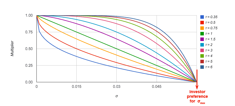
Now our measure, which we have dubbed the "Variability-Weighted Return", is the normalized logarithmic return times a multiplier, ranging from $0$ to $1$, that weights the fund's return by a factor corresponding to the investor's preference for price variability tolerance ($τ$).  This new measure contains far more information than the Sharpe Ratio.

Based on our observations, the curve representing typical investor preference for variability is similar to the curve in this chart with the exponent ($τ$) between 2 and 3.  Risk averse investors, such as those near or in retirement, may wish to choose a lower $σ_{max}$ and/or a risk tolerance ($τ$) of less than one.

So, how did we do?  Let's take a look at some charts, to see if these scores make sense.  First a daily price chart: Here are the normalized mean log returns and price-differential standard deviations experienced for the above funds, using daily, weekly, or monthly sub-periods:



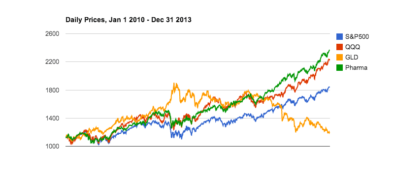
The first thing you may notice is that, unlike the values used in the Sharpe Ratio, the parameters we use are consistent for each fund, across daily, weekly, or monthly granularity.  Properly normalized returns would be identical for each sub-period length.  However, in our case, we used $52$ as the number of weeks per year, when, in our sample, we had $52.25$ weeks per year ($209$ sub-periods to cover all 4 years, with weekly closes).  We used $251.5$ trading days per year, which was correct during these 4 years.

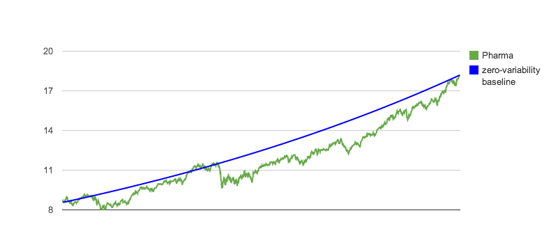
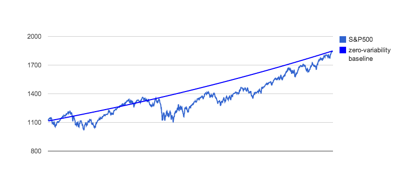
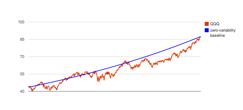
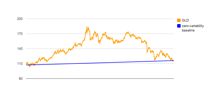
Before we continue, let's take a closer look at the 4 funds above, in relation to their zero-variability baselines, so their price variabilities become more obvious: How do these funds score using the VWR?  In this example, let's say we really do not want any fund much more volatile than GLD has been over the last 4 years.   So, we'll choose $σ_{max}$ to be $0.19$.  We will use $τ = 2$ for our variability tolerance.  For the Sharpe Ratio calculations, we will use a risk-free rate of 2.75%.  Here are the results:



Which values are more meaningful?  When a person tells us that a fund has a Sharpe Ratio of 0.0159, what does that tell us?  First, we must ask what was used for the benchmark in the calculations.  Then, we must ask about the granularity used.  Did they use daily values?  Weekly?  Monthly?  Yearly?  Even then, what does 0.0159 mean?  With the Variability Weighted Return (VWR), we at least can relate the value to an annual return rate, attenuated for variability.  In the case of the funds above, the Sharpe Ratio did put the funds in our order of preference, but what if we change our preferences, or the funds we are considering have a greater disparity of variability?

Notes: GLD has poor returns over this period, as well as the highest variability in the group.  So, it rightfully scores at the lowest value.  Since its $σ_P$ is very close to the $σ_{max}$ we have chosen, it will score close to zero, regardless of return.  The pharmaceutical fund has the highest return and, remarkably, the lowest $σ_P$ over this period.  So, it is properly scored at the highest of the set.  But, what if our preferences change?  Here is an interactive tool to use to experiment with $σ_{max}$ and $τ$ values, to see how the affect the scoring:



Below, we show an example where the Sharpe Ratio fails in properly scoring the funds.  Consider the following funds, in a weekly chart from 2010-2013:

Here are the VWR and Sharpe Ratio values:



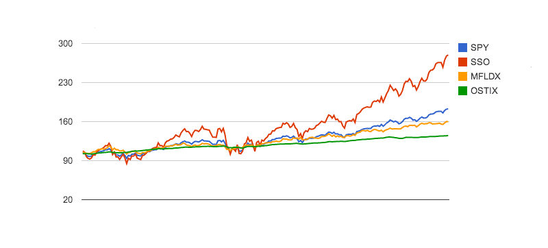
We find the Sharpe Ratio values completely unhelpful here.  Practically no discrimination is made between the low-return, low-volatility fund MFLDX, and the high-return, high-volatility fund SSO, even though these funds have wildly different characteristics.  This is one of the problems inherent in using a ratio.  Using the Sharpe Ratio, little discrimination is made between SPY and its 2x ETF cousin, SSO.  Because of its extremely low volatility (See: Standard Deviation ($σ$) does not belong in the denominator, above), the short-term bond fund OSTIX has a Sharpe Ratio of more than double the next closest fund, while few investors would have preferred this fund over this period of time.  Using the VWR, the scores fall in line with expectations, and one can adjust the preferences to penalize more heavily the volatility of SSO and SPY.  No such adjustments are available with Sharpe.

Let's take a closer look, so we can understand why the Sharpe Ratio is nearly identical for SSO and MFLDX:



As you can see, SSO had an $R↖{-}$  which was 3.02 times that of MFLDX.  But, it also had a $σ_D$  which was 3.03 times that of MFLDX.  Thus, their Sharpe Ratios are nearly identical.  We find the inability of the Sharpe ratio to distinguish between these 2 vastly different funds troubling, as this could lead investors to make choices which do not well serve their portfolios.  $R↖{-}$  for OSTIX approached zero during this period.  But, its Sharpe denominator $σ_D$  also approached zero, launching its Sharpe Ratio to the highest of the group.  Across this group of funds, the Sharpe Ratio has mislead the investor into incorrect scoring.  The VWR allows investors to choose weighting preferences for returns versus variability, which can more accurately target their desired performance.

OK, one last chart.  Let's take a look at the same funds, over a period which contains a market correction, to see how the indicators perform under more difficult conditions.  Here are the same four funds, from 2008-2013:

Here are the VWR and Sharpe Ratio values:



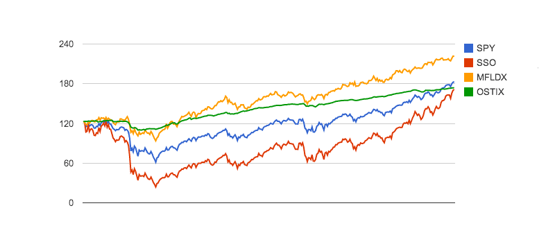
Again, the VWR does a much better job of scoring these funds than does the Sharpe Ratio.  Note that, because its $σ_P$  value, at 0.19107, was higher than the limit set in our preferences, SSO scored a zero using the VWR method.  Using Sharpe, SSO and SPY were virtually indistinguishable, and OSTIX still scores higher than the best fund of the group.

HINT: If you wish to consider funds with the variability of SSO, change the $σ_{max}$  value in the utility above to 0.2 or higher.  Then, adjust the $τ$  value to change your preference for variability weighting.  As you will see, VWR scores these funds in a much more valuable manner.  Here are the $R_{norm}$   and $σ_P$  values for your review:

What is proposed here is a more practical method of scoring funds, based on actual compounded returns and weighting for price variability.  It overcomes some of the fundamental problems inherent in the Sharpe Ratio.  Our new method, Variability-Weighted Return (VWR)  provides the following improvements:

1.  Weighting for returns is now representative of actual compounded returns.
   
2.  Weighting for variability in price is a better proxy for risk than variability in sub-periodic returns.
   
3.  Weighting for variability now matches observed investor behavior vis-a-vis price variability as risk.
   
4.  Weighting for variability can now be customized per investor preferences.
   
5.  Comparison to a benchmark fund is not required.
   
6.  Scoring is less dependent upon granularity of samples (time per sub-period), and more easily comparable to others.
   

For more aggressive stock traders who want stock symbols rather than a single score, pair this framework with our Stocks To Watch

We would love to hear your comments.   Email Us

Frequently asked questions

What is this page about?

It explains fundamental problems CrystalBull sees in Modern Portfolio Theory’s use of the Sharpe Ratio and introduces the Variability-Weighted Return (VWR) as a practical alternative scoring method using log returns and price-variability weighting.

Why prefer log returns in the numerator?

Periodic percentage returns are not additive; arithmetic means can label very different compounded outcomes as “the same.” Logarithmic returns are additive across sub-periods and map cleanly to total compounded growth, which CrystalBull then normalizes to a familiar annualized return figure.

How is VWR different from the Sharpe Ratio?

Sharpe divides average differential returns by the standard deviation of those returns. VWR multiplies a normalized log return by a variability weight between 0 and 1 based on how far prices wander from a constant-log-growth path, with investor-chosen limits (σ_max) and tolerance (τ)—avoiding infinite scores when volatility approaches zero.

Who is this for?

Investors, advisors, and researchers comparing funds or strategies on return versus variability—especially anyone who finds Sharpe rankings unintuitive across high-vol growers and low-vol low-return vehicles. CrystalBull also ties the motivation to how it thinks about return-versus-variability in its live timing stack.

What are the limitations?

VWR still relies on historical sample paths and user-chosen parameters (σ_max, τ); different choices change rankings. It does not remove market risk or forecast future returns. The article is educational methodology, not a certified performance composite or a trade signal.